New York Cty Airbnb Open Data
데이터 셋 : https://www.kaggle.com/dgomonov/new-york-city-airbnb-open-data
뉴욕시 에어비앤비에 전시된 여러 공간의 변수들을 통해 적당한 ‘이용료’를 파악-분류하고자 하는 데이터 셋이다.
라이브러리 설정 및 데이터 읽어들이기
import pandas as pd
import numpy as np
import seaborn as sns
import matplotlib.pyplot as plt

df = pd.read_csv('AB_NYC_2019.csv')

pd.set_option('display.max_columns', None)
df.head()
| id | name | host_id | host_name | neighbourhood_group | neighbourhood | latitude | longitude | room_type | price | minimum_nights | number_of_reviews | last_review | reviews_per_month | calculated_host_listings_count | availability_365 | |
|---|---|---|---|---|---|---|---|---|---|---|---|---|---|---|---|---|
| 0 | 2539 | Clean & quiet apt home by the park | 2787 | John | Brooklyn | Kensington | 40.64749 | -73.97237 | Private room | 149 | 1 | 9 | 2018-10-19 | 0.21 | 6 | 365 |
| 1 | 2595 | Skylit Midtown Castle | 2845 | Jennifer | Manhattan | Midtown | 40.75362 | -73.98377 | Entire home/apt | 225 | 1 | 45 | 2019-05-21 | 0.38 | 2 | 355 |
| 2 | 3647 | THE VILLAGE OF HARLEM....NEW YORK ! | 4632 | Elisabeth | Manhattan | Harlem | 40.80902 | -73.94190 | Private room | 150 | 3 | 0 | NaN | NaN | 1 | 365 |
| 3 | 3831 | Cozy Entire Floor of Brownstone | 4869 | LisaRoxanne | Brooklyn | Clinton Hill | 40.68514 | -73.95976 | Entire home/apt | 89 | 1 | 270 | 2019-07-05 | 4.64 | 1 | 194 |
| 4 | 5022 | Entire Apt: Spacious Studio/Loft by central park | 7192 | Laura | Manhattan | East Harlem | 40.79851 | -73.94399 | Entire home/apt | 80 | 10 | 9 | 2018-11-19 | 0.10 | 1 | 0 |
df.info()
<class 'pandas.core.frame.DataFrame'>
RangeIndex: 48895 entries, 0 to 48894
Data columns (total 16 columns):
 #   Column                          Non-Null Count  Dtype
---  ------                          --------------  -----
 0   id                              48895 non-null  int64
 1   name                            48879 non-null  object
 2   host_id                         48895 non-null  int64
 3   host_name                       48874 non-null  object
 4   neighbourhood_group             48895 non-null  object
 5   neighbourhood                   48895 non-null  object
 6   latitude                        48895 non-null  float64
 7   longitude                       48895 non-null  float64
 8   room_type                       48895 non-null  object
 9   price                           48895 non-null  int64
 10  minimum_nights                  48895 non-null  int64
 11  number_of_reviews               48895 non-null  int64
 12  last_review                     38843 non-null  object
 13  reviews_per_month               38843 non-null  float64
 14  calculated_host_listings_count  48895 non-null  int64
 15  availability_365                48895 non-null  int64
dtypes: float64(3), int64(7), object(6)
memory usage: 6.0+ MB
df.isna().sum()
id                                    0
name                                 16
host_id                               0
host_name                            21
neighbourhood_group                   0
neighbourhood                         0
latitude                              0
longitude                             0
room_type                             0
price                                 0
minimum_nights                        0
number_of_reviews                     0
last_review                       10052
reviews_per_month                 10052
calculated_host_listings_count        0
availability_365                      0
dtype: int64
- last_review 와 reviews_per_month 숫자가 같은것으로 보아 동일한 개수의 데이터일 듯 하다.
(df['number_of_reviews'] == 0).sum()
10052
- number of reviews가 0인 데이터가 10052인것으로 보아 해당 데이터가 last_review, reviews_per_month가 결측되어 있음을 알 수 있다.
# 곱셉 기능을 통해 True False 유무 확인. & 기능을 통해 True False 확인.
(df['reviews_per_month'].isna() & df['last_review'].isna()).sum()
10052
- 10052로 null 값 생성. 즉 두 변수가 가지고 있는 결측치의 인덱스가 동일
EDA 및 기초통계 분석
불필요한 column 제거
- ID, host_name, latitude, longitude은 직관적으로 가격에 영향을 및지 않을 것 같음. 위도와 경도의 경우 다를 수 있겠으나 일단 제거.
- name 역시 자연어 처리를 통해 유의미한 결과값을 뽑아낼 수 있겠으나 일단 EDA - 데이터 분석을 위해 제거.
- 리뷰관련된 변수의 경우 리뷰의 유무라는 새로운 변수 생성가능. 이용 가능 일수 역시 0일(이용 일수 미입력)이라는 변수 새롭게 생성 가능
df['room_type'].value_counts()
Entire home/apt    25409
Private room       22326
Shared room         1160
Name: room_type, dtype: int64
df['availability_365'].hist()
<matplotlib.axes._subplots.AxesSubplot at 0x269799e7508>

# 이용 가능 일수가 0인 데이터.

(df['availability_365'] == 0).sum()
17533
df.describe()
| id | host_id | latitude | longitude | price | minimum_nights | number_of_reviews | reviews_per_month | calculated_host_listings_count | availability_365 | |
|---|---|---|---|---|---|---|---|---|---|---|
| count | 4.889500e+04 | 4.889500e+04 | 48895.000000 | 48895.000000 | 48895.000000 | 48895.000000 | 48895.000000 | 38843.000000 | 48895.000000 | 48895.000000 |
| mean | 1.901714e+07 | 6.762001e+07 | 40.728949 | -73.952170 | 152.720687 | 7.029962 | 23.274466 | 1.373221 | 7.143982 | 112.781327 |
| std | 1.098311e+07 | 7.861097e+07 | 0.054530 | 0.046157 | 240.154170 | 20.510550 | 44.550582 | 1.680442 | 32.952519 | 131.622289 |
| min | 2.539000e+03 | 2.438000e+03 | 40.499790 | -74.244420 | 0.000000 | 1.000000 | 0.000000 | 0.010000 | 1.000000 | 0.000000 |
| 25% | 9.471945e+06 | 7.822033e+06 | 40.690100 | -73.983070 | 69.000000 | 1.000000 | 1.000000 | 0.190000 | 1.000000 | 0.000000 |
| 50% | 1.967728e+07 | 3.079382e+07 | 40.723070 | -73.955680 | 106.000000 | 3.000000 | 5.000000 | 0.720000 | 1.000000 | 45.000000 |
| 75% | 2.915218e+07 | 1.074344e+08 | 40.763115 | -73.936275 | 175.000000 | 5.000000 | 24.000000 | 2.020000 | 2.000000 | 227.000000 |
| max | 3.648724e+07 | 2.743213e+08 | 40.913060 | -73.712990 | 10000.000000 | 1250.000000 | 629.000000 | 58.500000 | 327.000000 | 365.000000 |
- 가격의 경우 최소가격과 최대가격의 설정이 잘못 되었다. 최소 숙박일수 역시 최대값이 잘못 설정되었다.
df.columns
Index(['id', 'name', 'host_id', 'host_name', 'neighbourhood_group',
       'neighbourhood', 'latitude', 'longitude', 'room_type', 'price',
       'minimum_nights', 'number_of_reviews', 'last_review',
       'reviews_per_month', 'calculated_host_listings_count',
       'availability_365'],
      dtype='object')
df.drop(['id', 'name', 'host_name', 'latitude', 'longitude'], axis=1, inplace=True)
df.head()
| host_id | neighbourhood_group | neighbourhood | room_type | price | minimum_nights | number_of_reviews | last_review | reviews_per_month | calculated_host_listings_count | availability_365 | |
|---|---|---|---|---|---|---|---|---|---|---|---|
| 0 | 2787 | Brooklyn | Kensington | Private room | 149 | 1 | 9 | 2018-10-19 | 0.21 | 6 | 365 |
| 1 | 2845 | Manhattan | Midtown | Entire home/apt | 225 | 1 | 45 | 2019-05-21 | 0.38 | 2 | 355 |
| 2 | 4632 | Manhattan | Harlem | Private room | 150 | 3 | 0 | NaN | NaN | 1 | 365 |
| 3 | 4869 | Brooklyn | Clinton Hill | Entire home/apt | 89 | 1 | 270 | 2019-07-05 | 4.64 | 1 | 194 |
| 4 | 7192 | Manhattan | East Harlem | Entire home/apt | 80 | 10 | 9 | 2018-11-19 | 0.10 | 1 | 0 |
수치형 데이터
- 수치형 데이터를 통해서만 price를 예측할 수 있을까?
sns.jointplot(data=df, x='reviews_per_month', y='price')
<seaborn.axisgrid.JointGrid at 0x2697ab33148>

sns.heatmap(df.corr(), annot=True, cmap='YlOrRd')
<matplotlib.axes._subplots.AxesSubplot at 0x2697b48fec8>
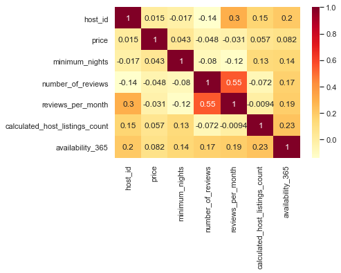
- 전처리가 되어 있지 않아서 상관성을 파악하기 어렵다.
- 의외로 host_id가 상관성이 있어보이는데 사용일수와 0.2, 한달동안 리뷰는 0.3 으로 확인할 수 있다.
- 새롭게 운영하는 사람일수록 큰 숫자의 id를 가지고 있고 새 시설인 만큼 리뷰도 많이 받고 오래 이용할 수 있기 때문인지 확인이 더 필요하다.
- host_id에 있어서 누적리뷰와 한달동안 받는 리뷰가 다른 상관성을 띈다.
범주형 데이터
sns.boxplot(data=df, x='neighbourhood_group', y='price')
<matplotlib.axes._subplots.AxesSubplot at 0x2697e22af08>

- 최대값이외에도 평균 기준값을 훨씬 초과하는 아웃라이어 price 값들이 있어서 확인하기 어렵다. 전처리 필요
데이터 전처리
범주형 데이터 전처리
df['neighbourhood_group'].value_counts()
Manhattan        21661
Brooklyn         20104
Queens            5666
Bronx             1091
Staten Island      373
Name: neighbourhood_group, dtype: int64
df['neighbourhood'].value_counts()
Williamsburg          3920
Bedford-Stuyvesant    3714
Harlem                2658
Bushwick              2465
Upper West Side       1971
                      ...
Woodrow                  1
Fort Wadsworth           1
New Dorp                 1
Richmondtown             1
Rossville                1
Name: neighbourhood, Length: 221, dtype: int64
plt.plot(range(len(df['neighbourhood'].value_counts())), df['neighbourhood'].value_counts())
[<matplotlib.lines.Line2D at 0x2697e315588>]
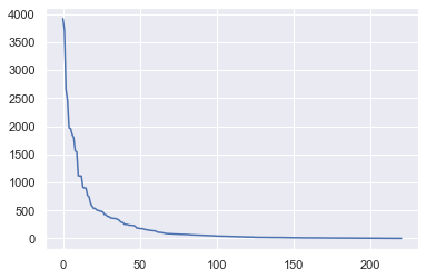
- 소수의 값 제거를 위해 50번째 이전 value 값만 잔존시킴.
ne = df['neighbourhood'].value_counts()[50:]
df['neighbourhood'] = df['neighbourhood'].apply(lambda s : s if str(s) not in ne[50:] else 'others')
수치형 데이터 전처리
sns.rugplot(data=df, x='price', height=1)
<matplotlib.axes._subplots.AxesSubplot at 0x2697e36a348>

print(df['price'].quantile(0.99))
print(df['price'].quantile(0.005))
799.0
26.0
- price값 상위 1% 가 799달러 즉, 1000달러 이후의 데이터는 아웃라이어 값으로 판단할 수 있다.
- price값 하위 아웃라이어 값 제거를 위해 0.5% 제거, 상위는 5% 제거
sns.rugplot(data=df, x='minimum_nights', height=1)
<matplotlib.axes._subplots.AxesSubplot at 0x2697e4aaf88>

print(df['minimum_nights'].quantile(0.98))
print(df['minimum_nights'].quantile(0.005))
30.0
1.0
- minimum_nights 경우 최소값은 자를 필요가 없고 상위 2%정도로 자르면 될 듯 하다.
sns.rugplot(data=df, x='availability_365', height=1)
<matplotlib.axes._subplots.AxesSubplot at 0x269028d0e88>
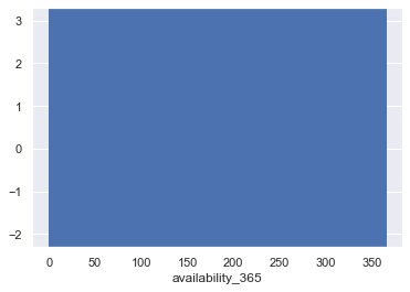
df['availability_365'].quantile(0.3)
0.0
- 30% 까지 0이라는 것은 미입력된 데이터가 상당하다는 뜻으로 차라리 이용일수가’0’인 새로운 범주형변수를 생성하는것이 효율적으로 보인다.
p1= df['price'].quantile(0.95)
p2= df['price'].quantile(0.005)

df = df[(p1 > df['price']) & (df['price'] > p2)]
df['price'].hist()
<matplotlib.axes._subplots.AxesSubplot at 0x269042e5fc8>

df['minimum_nights'].quantile(0.98)
30.0
- price에서 아웃라이어 제거해도 상위 2%값 변하지 않음. 그대로 진행해도 좋다.
m1 = df['minimum_nights'].quantile(0.98)
df = df[df['minimum_nights'] < m1 ]
from sklearn.preprocessing import StandardScaler
scaler = StandardScaler()
X_num = df.drop(['neighbourhood_group', 'neighbourhood', 'room_type', 'avail_zero', 'review_exists','last_review','price'], axis=1)

scaler.fit(X_num)
X_scaled = scaler.transform(X_num)
X_scaled = pd.DataFrame(X_scaled, index=X_num.index, columns=X_num.columns)

# last_review 경우 수치형이긴 하지만 날짜형태
범주형 데이터 전처리
# availability_365 중 새로운 범주형 변수 생성

df['avail_zero'] = df['availability_365'].apply(lambda x : 'Zero' if x==0 else 'NonZero')
# review 중 Null 값 채우기.

df['review_exists'] = df['reviews_per_month'].isna().apply(lambda x: 'No' if x is True else 'Yes')

df.fillna(0, inplace=True) # 현재 미기입은 리뷰만 있음.
df.columns
Index(['host_id', 'neighbourhood_group', 'neighbourhood', 'room_type', 'price',
       'minimum_nights', 'number_of_reviews', 'last_review',
       'reviews_per_month', 'calculated_host_listings_count',
       'availability_365', 'avail_zero', 'review_exists'],
      dtype='object')
X_cat = df[['neighbourhood_group', 'neighbourhood', 'room_type', 'avail_zero', 'review_exists']]
X_cat = pd.get_dummies(X_cat)

# 선형회귀일 경우 get dummies 실행시 drop_first 그라디언트 부스트 사용시 X.
X = pd.concat([X_scaled, X_cat], axis=1)
y = df['price']
X.head()
| host_id | minimum_nights | number_of_reviews | reviews_per_month | calculated_host_listings_count | availability_365 | neighbourhood_group_Bronx | neighbourhood_group_Brooklyn | neighbourhood_group_Manhattan | neighbourhood_group_Queens | neighbourhood_group_Staten Island | neighbourhood_Arverne | neighbourhood_Astoria | neighbourhood_Battery Park City | neighbourhood_Bay Ridge | neighbourhood_Bedford-Stuyvesant | neighbourhood_Bensonhurst | neighbourhood_Boerum Hill | neighbourhood_Borough Park | neighbourhood_Briarwood | neighbourhood_Brighton Beach | neighbourhood_Brooklyn Heights | neighbourhood_Brownsville | neighbourhood_Bushwick | neighbourhood_Canarsie | neighbourhood_Carroll Gardens | neighbourhood_Chelsea | neighbourhood_Chinatown | neighbourhood_Civic Center | neighbourhood_Clinton Hill | neighbourhood_Cobble Hill | neighbourhood_Concourse | neighbourhood_Corona | neighbourhood_Crown Heights | neighbourhood_Cypress Hills | neighbourhood_Ditmars Steinway | neighbourhood_Downtown Brooklyn | neighbourhood_East Elmhurst | neighbourhood_East Flatbush | neighbourhood_East Harlem | neighbourhood_East New York | neighbourhood_East Village | neighbourhood_Elmhurst | neighbourhood_Financial District | neighbourhood_Flatbush | neighbourhood_Flatiron District | neighbourhood_Flatlands | neighbourhood_Flushing | neighbourhood_Fordham | neighbourhood_Forest Hills | neighbourhood_Fort Greene | neighbourhood_Fort Hamilton | neighbourhood_Glendale | neighbourhood_Gowanus | neighbourhood_Gramercy | neighbourhood_Gravesend | neighbourhood_Greenpoint | neighbourhood_Greenwich Village | neighbourhood_Harlem | neighbourhood_Hell's Kitchen | neighbourhood_Inwood | neighbourhood_Jackson Heights | neighbourhood_Jamaica | neighbourhood_Kensington | neighbourhood_Kingsbridge | neighbourhood_Kips Bay | neighbourhood_Little Italy | neighbourhood_Long Island City | neighbourhood_Longwood | neighbourhood_Lower East Side | neighbourhood_Maspeth | neighbourhood_Midtown | neighbourhood_Midwood | neighbourhood_Morningside Heights | neighbourhood_Mott Haven | neighbourhood_Murray Hill | neighbourhood_NoHo | neighbourhood_Nolita | neighbourhood_Ozone Park | neighbourhood_Park Slope | neighbourhood_Port Morris | neighbourhood_Prospect Heights | neighbourhood_Prospect-Lefferts Gardens | neighbourhood_Queens Village | neighbourhood_Red Hook | neighbourhood_Rego Park | neighbourhood_Richmond Hill | neighbourhood_Ridgewood | neighbourhood_Rockaway Beach | neighbourhood_Roosevelt Island | neighbourhood_Rosedale | neighbourhood_Sheepshead Bay | neighbourhood_SoHo | neighbourhood_South Slope | neighbourhood_Springfield Gardens | neighbourhood_St. Albans | neighbourhood_St. George | neighbourhood_Sunnyside | neighbourhood_Sunset Park | neighbourhood_Theater District | neighbourhood_Tribeca | neighbourhood_Two Bridges | neighbourhood_Upper East Side | neighbourhood_Upper West Side | neighbourhood_Wakefield | neighbourhood_Washington Heights | neighbourhood_West Village | neighbourhood_Williamsburg | neighbourhood_Windsor Terrace | neighbourhood_Woodhaven | neighbourhood_Woodside | neighbourhood_others | room_type_Entire home/apt | room_type_Private room | room_type_Shared room | avail_zero_NonZero | avail_zero_Zero | review_exists_No | review_exists_Yes | |
|---|---|---|---|---|---|---|---|---|---|---|---|---|---|---|---|---|---|---|---|---|---|---|---|---|---|---|---|---|---|---|---|---|---|---|---|---|---|---|---|---|---|---|---|---|---|---|---|---|---|---|---|---|---|---|---|---|---|---|---|---|---|---|---|---|---|---|---|---|---|---|---|---|---|---|---|---|---|---|---|---|---|---|---|---|---|---|---|---|---|---|---|---|---|---|---|---|---|---|---|---|---|---|---|---|---|---|---|---|---|---|---|---|---|---|---|---|---|---|---|
| 0 | -0.848227 | -0.588004 | -0.352358 | -0.588299 | 0.066069 | 2.132586 | 0 | 1 | 0 | 0 | 0 | 0 | 0 | 0 | 0 | 0 | 0 | 0 | 0 | 0 | 0 | 0 | 0 | 0 | 0 | 0 | 0 | 0 | 0 | 0 | 0 | 0 | 0 | 0 | 0 | 0 | 0 | 0 | 0 | 0 | 0 | 0 | 0 | 0 | 0 | 0 | 0 | 0 | 0 | 0 | 0 | 0 | 0 | 0 | 0 | 0 | 0 | 0 | 0 | 0 | 0 | 0 | 0 | 1 | 0 | 0 | 0 | 0 | 0 | 0 | 0 | 0 | 0 | 0 | 0 | 0 | 0 | 0 | 0 | 0 | 0 | 0 | 0 | 0 | 0 | 0 | 0 | 0 | 0 | 0 | 0 | 0 | 0 | 0 | 0 | 0 | 0 | 0 | 0 | 0 | 0 | 0 | 0 | 0 | 0 | 0 | 0 | 0 | 0 | 0 | 0 | 0 | 0 | 1 | 0 | 1 | 0 | 0 | 1 |
| 1 | -0.848227 | -0.588004 | 0.419649 | -0.485721 | -0.084134 | 2.052616 | 0 | 0 | 1 | 0 | 0 | 0 | 0 | 0 | 0 | 0 | 0 | 0 | 0 | 0 | 0 | 0 | 0 | 0 | 0 | 0 | 0 | 0 | 0 | 0 | 0 | 0 | 0 | 0 | 0 | 0 | 0 | 0 | 0 | 0 | 0 | 0 | 0 | 0 | 0 | 0 | 0 | 0 | 0 | 0 | 0 | 0 | 0 | 0 | 0 | 0 | 0 | 0 | 0 | 0 | 0 | 0 | 0 | 0 | 0 | 0 | 0 | 0 | 0 | 0 | 0 | 1 | 0 | 0 | 0 | 0 | 0 | 0 | 0 | 0 | 0 | 0 | 0 | 0 | 0 | 0 | 0 | 0 | 0 | 0 | 0 | 0 | 0 | 0 | 0 | 0 | 0 | 0 | 0 | 0 | 0 | 0 | 0 | 0 | 0 | 0 | 0 | 0 | 0 | 0 | 0 | 0 | 1 | 0 | 0 | 1 | 0 | 0 | 1 |
| 2 | -0.848204 | -0.119342 | -0.545360 | -0.715013 | -0.121684 | 2.132586 | 0 | 0 | 1 | 0 | 0 | 0 | 0 | 0 | 0 | 0 | 0 | 0 | 0 | 0 | 0 | 0 | 0 | 0 | 0 | 0 | 0 | 0 | 0 | 0 | 0 | 0 | 0 | 0 | 0 | 0 | 0 | 0 | 0 | 0 | 0 | 0 | 0 | 0 | 0 | 0 | 0 | 0 | 0 | 0 | 0 | 0 | 0 | 0 | 0 | 0 | 0 | 0 | 1 | 0 | 0 | 0 | 0 | 0 | 0 | 0 | 0 | 0 | 0 | 0 | 0 | 0 | 0 | 0 | 0 | 0 | 0 | 0 | 0 | 0 | 0 | 0 | 0 | 0 | 0 | 0 | 0 | 0 | 0 | 0 | 0 | 0 | 0 | 0 | 0 | 0 | 0 | 0 | 0 | 0 | 0 | 0 | 0 | 0 | 0 | 0 | 0 | 0 | 0 | 0 | 0 | 0 | 0 | 1 | 0 | 1 | 0 | 1 | 0 |
| 3 | -0.848200 | -0.588004 | 5.244692 | 2.084766 | -0.121684 | 0.765095 | 0 | 1 | 0 | 0 | 0 | 0 | 0 | 0 | 0 | 0 | 0 | 0 | 0 | 0 | 0 | 0 | 0 | 0 | 0 | 0 | 0 | 0 | 0 | 1 | 0 | 0 | 0 | 0 | 0 | 0 | 0 | 0 | 0 | 0 | 0 | 0 | 0 | 0 | 0 | 0 | 0 | 0 | 0 | 0 | 0 | 0 | 0 | 0 | 0 | 0 | 0 | 0 | 0 | 0 | 0 | 0 | 0 | 0 | 0 | 0 | 0 | 0 | 0 | 0 | 0 | 0 | 0 | 0 | 0 | 0 | 0 | 0 | 0 | 0 | 0 | 0 | 0 | 0 | 0 | 0 | 0 | 0 | 0 | 0 | 0 | 0 | 0 | 0 | 0 | 0 | 0 | 0 | 0 | 0 | 0 | 0 | 0 | 0 | 0 | 0 | 0 | 0 | 0 | 0 | 0 | 0 | 1 | 0 | 0 | 1 | 0 | 0 | 1 |
| 4 | -0.848170 | 1.520973 | -0.352358 | -0.654673 | -0.121684 | -0.786327 | 0 | 0 | 1 | 0 | 0 | 0 | 0 | 0 | 0 | 0 | 0 | 0 | 0 | 0 | 0 | 0 | 0 | 0 | 0 | 0 | 0 | 0 | 0 | 0 | 0 | 0 | 0 | 0 | 0 | 0 | 0 | 0 | 0 | 1 | 0 | 0 | 0 | 0 | 0 | 0 | 0 | 0 | 0 | 0 | 0 | 0 | 0 | 0 | 0 | 0 | 0 | 0 | 0 | 0 | 0 | 0 | 0 | 0 | 0 | 0 | 0 | 0 | 0 | 0 | 0 | 0 | 0 | 0 | 0 | 0 | 0 | 0 | 0 | 0 | 0 | 0 | 0 | 0 | 0 | 0 | 0 | 0 | 0 | 0 | 0 | 0 | 0 | 0 | 0 | 0 | 0 | 0 | 0 | 0 | 0 | 0 | 0 | 0 | 0 | 0 | 0 | 0 | 0 | 0 | 0 | 0 | 1 | 0 | 0 | 0 | 1 | 0 | 1 |
학습 및 테스트 데이터 분리
from sklearn.model_selection import train_test_split
X_train, X_test, y_train, y_test = train_test_split(X, y, test_size=0.3, random_state=1)
분류하기 - XGBoost Regression 모델 적용
from xgboost import XGBRegressor

model_reg =XGBRegressor()
model_reg.fit(X_train, y_train)
XGBRegressor(base_score=0.5, booster='gbtree', colsample_bylevel=1,
             colsample_bynode=1, colsample_bytree=1, gamma=0, gpu_id=-1,
             importance_type='gain', interaction_constraints='',
             learning_rate=0.300000012, max_delta_step=0, max_depth=6,
             min_child_weight=1, missing=nan, monotone_constraints='()',
             n_estimators=100, n_jobs=4, num_parallel_tree=1,
             objective='reg:squarederror', random_state=0, reg_alpha=0,
             reg_lambda=1, scale_pos_weight=1, subsample=1, tree_method='exact',
             validate_parameters=1, verbosity=None)
모델 평가
from sklearn.metrics import mean_absolute_error, mean_squared_error
from math import sqrt

pred = model_reg.predict(X_test)
print(mean_absolute_error(y_test, pred))
print(sqrt(mean_squared_error(y_test, pred)))
34.158105898456235
48.339277624918665
- 낮은 값인지 높은값인지 직관적으로 쉬이 알기 어렵다.
plt.scatter(x=y_test, y=pred, alpha=0.1)
plt.plot([0,350], [0,350], 'r-')
[<matplotlib.lines.Line2D at 0x26907658148>]

- price 값의 경우 단위별로 나누어져 있는 경우가 많아 구간별로 나누어진다.
- 값이 낮을때는 overestimate 높을 경우는 underestimate 하는 현상이 일어남.
err = (pred - y_test) / y_test
sns.histplot(err)
plt.grid()
