Used Cars Dataset
데이터 셋 : https://www.kaggle.com/austinreese/craigslist-carstrucks-data
중고차가 가진 여러가지 변수를 통해 중고차의 가격을 예측하고자 하는 데이터 셋이다.
라이브러리 설정 및 데이터 읽어들이기
import pandas as pd
import numpy as np
import seaborn as sns
import matplotlib.pyplot as plt

df = pd.read_csv('vehicles.csv')

pd.set_option('display.max_columns', None)
df.head()
| Unnamed: 0 | id | url | region | region_url | price | year | manufacturer | model | condition | cylinders | fuel | odometer | title_status | transmission | VIN | drive | size | type | paint_color | image_url | description | state | lat | long | posting_date | |
|---|---|---|---|---|---|---|---|---|---|---|---|---|---|---|---|---|---|---|---|---|---|---|---|---|---|---|
| 0 | 0 | 7240372487 | https://auburn.craigslist.org/ctd/d/auburn-uni... | auburn | https://auburn.craigslist.org | 35990 | 2010.0 | chevrolet | corvette grand sport | good | 8 cylinders | gas | 32742.0 | clean | other | 1G1YU3DW1A5106980 | rwd | NaN | other | NaN | https://images.craigslist.org/00N0N_ipkbHVZYf4... | Carvana is the safer way to buy a car During t... | al | 32.590000 | -85.480000 | 2020-12-02T08:11:30-0600 |
| 1 | 1 | 7240309422 | https://auburn.craigslist.org/cto/d/auburn-201... | auburn | https://auburn.craigslist.org | 7500 | 2014.0 | hyundai | sonata | excellent | 4 cylinders | gas | 93600.0 | clean | automatic | 5NPEC4AB0EH813529 | fwd | NaN | sedan | NaN | https://images.craigslist.org/00s0s_gBHYmJ5o7y... | I'll move to another city and try to sell my c... | al | 32.547500 | -85.468200 | 2020-12-02T02:11:50-0600 |
| 2 | 2 | 7240224296 | https://auburn.craigslist.org/cto/d/auburn-200... | auburn | https://auburn.craigslist.org | 4900 | 2006.0 | bmw | x3 3.0i | good | 6 cylinders | gas | 87046.0 | clean | automatic | NaN | NaN | NaN | SUV | blue | https://images.craigslist.org/00B0B_5zgEGWPOrt... | Clean 2006 BMW X3 3.0I. Beautiful and rare Bl... | al | 32.616807 | -85.464149 | 2020-12-01T19:50:41-0600 |
| 3 | 3 | 7240103965 | https://auburn.craigslist.org/cto/d/lanett-tru... | auburn | https://auburn.craigslist.org | 2000 | 1974.0 | chevrolet | c-10 | good | 4 cylinders | gas | 190000.0 | clean | automatic | NaN | rwd | full-size | pickup | blue | https://images.craigslist.org/00M0M_6o7KcDpArw... | 1974 chev. truck (LONG BED) NEW starter front ... | al | 32.861600 | -85.216100 | 2020-12-01T15:54:45-0600 |
| 4 | 4 | 7239983776 | https://auburn.craigslist.org/cto/d/auburn-200... | auburn | https://auburn.craigslist.org | 19500 | 2005.0 | ford | f350 lariat | excellent | 8 cylinders | diesel | 116000.0 | lien | automatic | NaN | 4wd | full-size | pickup | blue | https://images.craigslist.org/00p0p_b95l1EgUfl... | 2005 Ford F350 Lariat (Bullet Proofed). This t... | al | 32.547500 | -85.468200 | 2020-12-01T12:53:56-0600 |
df.info()
<class 'pandas.core.frame.DataFrame'>
RangeIndex: 458213 entries, 0 to 458212
Data columns (total 26 columns):
 #   Column        Non-Null Count   Dtype
---  ------        --------------   -----
 0   Unnamed: 0    458213 non-null  int64
 1   id            458213 non-null  int64
 2   url           458213 non-null  object
 3   region        458213 non-null  object
 4   region_url    458213 non-null  object
 5   price         458213 non-null  int64
 6   year          457163 non-null  float64
 7   manufacturer  439993 non-null  object
 8   model         453367 non-null  object
 9   condition     265273 non-null  object
 10  cylinders     287073 non-null  object
 11  fuel          454976 non-null  object
 12  odometer      402910 non-null  float64
 13  title_status  455636 non-null  object
 14  transmission  455771 non-null  object
 15  VIN           270664 non-null  object
 16  drive         324025 non-null  object
 17  size          136865 non-null  object
 18  type          345475 non-null  object
 19  paint_color   317370 non-null  object
 20  image_url     458185 non-null  object
 21  description   458143 non-null  object
 22  state         458213 non-null  object
 23  lat           450765 non-null  float64
 24  long          450765 non-null  float64
 25  posting_date  458185 non-null  object
dtypes: float64(4), int64(3), object(19)
memory usage: 90.9+ MB
EDA 및 기초 통계 분석
df.isna().sum()
Unnamed: 0           0
id                   0
url                  0
region               0
region_url           0
price                0
year              1050
manufacturer     18220
model             4846
condition       192940
cylinders       171140
fuel              3237
odometer         55303
title_status      2577
transmission      2442
VIN             187549
drive           134188
size            321348
type            112738
paint_color     140843
image_url           28
description         70
state                0
lat               7448
long              7448
posting_date        28
dtype: int64
df.describe()
| Unnamed: 0 | id | price | year | odometer | lat | long | |
|---|---|---|---|---|---|---|---|
| count | 458213.000000 | 4.582130e+05 | 4.582130e+05 | 457163.000000 | 4.029100e+05 | 450765.000000 | 450765.000000 |
| mean | 229106.000000 | 7.235233e+09 | 4.042093e+04 | 2010.746067 | 1.016698e+05 | 38.531925 | -94.375824 |
| std | 132274.843786 | 4.594362e+06 | 8.194599e+06 | 8.868136 | 3.228623e+06 | 5.857378 | 18.076225 |
| min | 0.000000 | 7.208550e+09 | 0.000000e+00 | 1900.000000 | 0.000000e+00 | -82.607549 | -164.091797 |
| 25% | 114553.000000 | 7.231953e+09 | 4.900000e+03 | 2008.000000 | 4.087700e+04 | 34.600000 | -110.890427 |
| 50% | 229106.000000 | 7.236409e+09 | 1.099500e+04 | 2013.000000 | 8.764100e+04 | 39.244500 | -88.314889 |
| 75% | 343659.000000 | 7.239321e+09 | 2.149500e+04 | 2016.000000 | 1.340000e+05 | 42.484503 | -81.015022 |
| max | 458212.000000 | 7.241019e+09 | 3.615215e+09 | 2021.000000 | 2.043756e+09 | 82.049255 | 150.898969 |
- 가격/ 평균값이 4만달러, 중위값이 천만달러
- 가격 /최소값이 0, 최대값이 터무니없이 높음(잘못설정된것(아웃라이어))
- 주행거리 역시 잘못된 데이터가 있음.
불필요한 column 제거
- year를 연식(age)값으로 바꿈.
df.columns
Index(['Unnamed: 0', 'id', 'url', 'region', 'region_url', 'price', 'year',
       'manufacturer', 'model', 'condition', 'cylinders', 'fuel', 'odometer',
       'title_status', 'transmission', 'VIN', 'drive', 'size', 'type',
       'paint_color', 'image_url', 'description', 'state', 'lat', 'long',
       'posting_date'],
      dtype='object')
df.drop(['Unnamed: 0', 'id', 'url', 'region_url', 'VIN',
         'image_url', 'description', 'state', 'lat', 'long',
         'posting_date'], axis=1, inplace=True)
df['age'] = 2021 - df['year']
df.drop('year', axis=1, inplace=True)
범주형 데이터 분석
len(df['manufacturer'].value_counts())
43
plt.figure(figsize=(8,10))
sns.countplot(data=df.fillna('n/a'), y='manufacturer', order=df.fillna('n/a')['manufacturer'].value_counts().index)
<matplotlib.axes._subplots.AxesSubplot at 0x1c5b58bfb88>

len(df['model'].value_counts())

# for model, num in zip(df['model'].value_counts().index df['model'].value_counts()):
# print(model, num)
31520
len(df['condition'].value_counts())
6
len(df['cylinders'].value_counts())
8
sns.countplot(data=df.fillna('n/a'), y='transmission', order=df.fillna('n/a')['transmission'].value_counts().index)
<matplotlib.axes._subplots.AxesSubplot at 0x1c5b5961c08>

sns.countplot(data=df.fillna('n/a'), y='drive', order=df.fillna('n/a')['drive'].value_counts().index)
<matplotlib.axes._subplots.AxesSubplot at 0x1c5b594f788>

sns.countplot(data=df.fillna('n/a'), y='size', order=df.fillna('n/a')['size'].value_counts().index)
<matplotlib.axes._subplots.AxesSubplot at 0x1c5ba1cfc88>

sns.countplot(data=df.fillna('n/a'), y='type', order=df.fillna('n/a')['type'].value_counts().index)
<matplotlib.axes._subplots.AxesSubplot at 0x1c5b9daf8c8>

sns.countplot(data=df.fillna('n/a'), y='paint_color', order=df.fillna('n/a')['paint_color'].value_counts().index)
<matplotlib.axes._subplots.AxesSubplot at 0x1c5a9223d88>

수치형 데이터 분석
df.columns
Index(['region', 'price', 'manufacturer', 'model', 'condition', 'cylinders',
       'fuel', 'odometer', 'title_status', 'transmission', 'drive', 'size',
       'type', 'paint_color', 'age'],
      dtype='object')
plt.figure(figsize=(8,2))
sns.rugplot(data=df, x='odometer', height=1)
<matplotlib.axes._subplots.AxesSubplot at 0x1c5b4522d48>

sns.histplot(data=df, x='age', bins=20, kde=True)
<matplotlib.axes._subplots.AxesSubplot at 0x1c59ed64a48>

데이터 전처리
범주형 데이터 전처리
sns.boxplot(data=df.fillna('n/a'), x='manufacturer', y='price')
<matplotlib.axes._subplots.AxesSubplot at 0x1c5b5162c48>

- 아웃라이어가 심각
df.columns
Index(['region', 'price', 'manufacturer', 'model', 'condition', 'cylinders',
       'fuel', 'odometer', 'title_status', 'transmission', 'drive', 'size',
       'type', 'paint_color', 'age'],
      dtype='object')
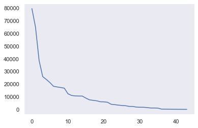
- 해당 Columns 들이 어느정도까지가 유의미한 데이터인지 확인하기 위해 plot를 그림.
col= 'manufacturer'
counts = df[col].fillna('others').value_counts()
plt.grid()
plt.plot(range(len(counts)), counts)

# 10 정도가 적당해보임.
[<matplotlib.lines.Line2D at 0x1c6857feec8>]
# 상위 10개에 포함되지 않는 분류의 경우 others로 취급
n_categorical = 10
counts.index[n_categorical:]
df[col] = df[col].apply(lambda s : s if str(s) not in counts.index[n_categorical:] else 'others')
df['manufacturer'].value_counts()
others       134392
ford          79666
chevrolet     64977
toyota        38577
honda         25868
nissan        23654
jeep          21165
ram           17697
gmc           17267
dodge         16730
Name: manufacturer, dtype: int64
col= 'model'
counts = df[col].fillna('others').value_counts()
plt.grid()
plt.plot(range(len(counts)), counts)
[<matplotlib.lines.Line2D at 0x1c684f1e808>]

col= 'model'
counts = df[col].fillna('others').value_counts()
plt.grid()
plt.plot(range(len(counts[:20])), counts[:20])
[<matplotlib.lines.Line2D at 0x1c684fad2c8>]

# manufacturer 와 달리 분류가 엄청 많아서 lambda 실행으로 느리게 작동할 수 있음.
n_categorical = 10
#counts.index[n_categorical:]
# df[col] = df[col].apply(lambda s : s if str(s) not in counts.index[n_categorical:] else 'others')
others = counts.index[n_categorical:]
df[col] = df[col].apply(lambda s : s if str(s) not in others else 'others')

df['model'].value_counts()
others            413556
f-150               8370
silverado 1500      5964
1500                4211
camry               4033
accord              3730
altima              3490
civic               3479
escape              3444
silverado           3090
Name: model, dtype: int64
col = 'condition'
counts = df[col].fillna('others').value_counts()
n_categorical = 3
others = counts.index[n_categorical:]
df[col] = df[col].apply(lambda s : s if str(s) not in others else 'others')
col = 'cylinders'
counts = df[col].fillna('others').value_counts()
n_categorical = 4
others = counts.index[n_categorical:]
df[col] = df[col].apply(lambda s : s if str(s) not in others else 'others')
col = 'fuel'
# counts = df[col].fillna('others').value_counts()
# counts.index

n_categorical = 2
others = counts.index[n_categorical:]
df[col] = df[col].apply(lambda s : s if str(s) not in others else 'others')
df.drop('title_status', axis=1, inplace=True)
col = 'transmission'
counts = df[col].fillna('others').value_counts()
n_categorical = 3
others = counts.index[n_categorical:]
df[col] = df[col].apply(lambda s : s if str(s) not in others else 'others')
col = 'drive'
df[col].fillna('others', inplace=True)
col = 'size'
counts = df[col].fillna('others').value_counts()
n_categorical = 2
others = counts.index[n_categorical:]
df[col] = df[col].apply(lambda s : s if str(s) not in others else 'others')
col = 'type'
counts = df[col].fillna('others').value_counts()
n_categorical = 8
others = counts.index[n_categorical:]
df[col] = df[col].apply(lambda s : s if str(s) not in others else 'others')

df.loc[df[col] == 'other', col] = 'others'

# other이란 분류도 있어서 others에 편입.
col = 'paint_color'
counts = df[col].fillna('others').value_counts()
n_categorical = 7
others = counts.index[n_categorical:]
df[col] = df[col].apply(lambda s : s if str(s) not in others else 'others')
수치형 데이터 전처리
# age는 양호, odometer와 price 조정 필요.
p1 = df['price'].quantile(0.99)
p2 = df['price'].quantile(0.1)
print(p1, p2)

# 가격 = 상위 1% , 하위 10%를 제거하여 아웃라이어 제거.
59900.0 651.0
df = df[(p1 > df['price']) & (df['price'] > p2)]
o1 = df['odometer'].quantile(0.99)
o2 = df['odometer'].quantile(0.1)
print(o1, o2)

# 주행거리 = 상위, 하위 1% 제거하여 아웃라이어 제거.
270000.0 17553.0
df = df[(o1 > df['odometer']) & (df['odometer'] > o2)]
df.describe()

# 아웃라이어 제거 하여 수치형 데이터 개괄
| price | odometer | age | |
|---|---|---|---|
| count | 324382.000000 | 324382.000000 | 323860.000000 |
| mean | 15314.530106 | 102569.319602 | 10.174001 |
| std | 11298.917484 | 55165.135400 | 7.076283 |
| min | 652.000000 | 17555.000000 | 0.000000 |
| 25% | 6500.000000 | 56199.000000 | 5.000000 |
| 50% | 12388.000000 | 98146.000000 | 9.000000 |
| 75% | 21000.000000 | 140482.750000 | 13.000000 |
| max | 59895.000000 | 269930.000000 | 121.000000 |
plt.figure(figsize=(10,8))
sns.boxplot(data=df, x='manufacturer', y='price')
<matplotlib.axes._subplots.AxesSubplot at 0x1c684c59cc8>

- 전체적인 범위가 다르지 않지만 평균 값들을 비교할 만하다.
plt.figure(figsize=(10,8))
sns.boxplot(data=df, x='model', y='price')
<matplotlib.axes._subplots.AxesSubplot at 0x1c684c6db08>

- 같은 모델이라도 상태, 주행거리에 따라 가격이 크게 달라짐. 물론 모델마다 다르기도함.
sns.heatmap(df.corr(), annot=True, cmap='YlOrRd')
<matplotlib.axes._subplots.AxesSubplot at 0x1c684ef1408>
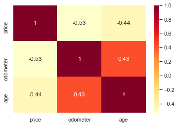
- 상관성은 높으나 주행거리, 연식 둘다 가격에 역방향으로 영향을 줌.
- 주행거리와 연식도 당연하게도 영향이 있음.
- 두개 모두 사용하면 비효율적인 모델이 될 수 있음.
from sklearn.preprocessing import StandardScaler

X_num = df[['odometer', 'age']]

scaler = StandardScaler()
scaler.fit(X_num)
X_scaled = scaler.transform(X_num)
X_scaled = pd.DataFrame(X_scaled, index=X_num.index, columns=X_num.columns)

# 범주형 데이터 one-hot 벡터로
X_cat = df.drop(['price', 'odometer', 'age'], axis=1)
X_cat = pd.get_dummies(X_cat)

X = pd.concat([X_scaled, X_cat], axis=1)
y = df['price']
X.head()
| odometer | age | region_SF bay area | region_abilene | region_akron / canton | region_albany | region_albuquerque | region_altoona-johnstown | region_amarillo | region_ames | region_anchorage / mat-su | region_ann arbor | region_annapolis | region_appleton-oshkosh-FDL | region_asheville | region_ashtabula | region_athens | region_atlanta | region_auburn | region_augusta | region_austin | region_bakersfield | region_baltimore | region_baton rouge | region_battle creek | region_beaumont / port arthur | region_bellingham | region_bemidji | region_bend | region_billings | region_binghamton | region_birmingham | region_bismarck | region_bloomington | region_bloomington-normal | region_boise | region_boone | region_boston | region_boulder | region_bowling green | region_bozeman | region_brainerd | region_brownsville | region_brunswick | region_buffalo | region_butte | region_cape cod / islands | region_catskills | region_cedar rapids | region_central NJ | region_central louisiana | region_central michigan | region_champaign urbana | region_charleston | region_charlotte | region_charlottesville | region_chattanooga | region_chautauqua | region_chicago | region_chico | region_chillicothe | region_cincinnati | region_clarksville | region_cleveland | region_clovis / portales | region_college station | region_colorado springs | region_columbia | region_columbia / jeff city | region_columbus | region_cookeville | region_corpus christi | region_corvallis/albany | region_cumberland valley | region_dallas / fort worth | region_danville | region_dayton / springfield | region_daytona beach | region_decatur | region_deep east texas | region_del rio / eagle pass | region_delaware | region_denver | region_des moines | region_detroit metro | region_dothan | region_dubuque | region_duluth / superior | region_east idaho | region_east oregon | region_eastern CO | region_eastern CT | region_eastern NC | region_eastern kentucky | region_eastern montana | region_eastern panhandle | region_eastern shore | region_eau claire | region_el paso | region_elko | region_elmira-corning | region_erie | region_eugene | region_evansville | region_fairbanks | region_fargo / moorhead | region_farmington | region_fayetteville | region_finger lakes | region_flagstaff / sedona | region_flint | region_florence | region_florence / muscle shoals | region_florida keys | region_fort collins / north CO | region_fort dodge | region_fort smith | region_fort smith, AR | region_fort wayne | region_frederick | region_fredericksburg | region_fresno / madera | region_ft myers / SW florida | region_gadsden-anniston | region_gainesville | region_galveston | region_glens falls | region_gold country | region_grand forks | region_grand island | region_grand rapids | region_great falls | region_green bay | region_greensboro | region_greenville / upstate | region_gulfport / biloxi | region_hanford-corcoran | region_harrisburg | region_harrisonburg | region_hartford | region_hattiesburg | region_hawaii | region_heartland florida | region_helena | region_hickory / lenoir | region_high rockies | region_hilton head | region_holland | region_houma | region_houston | region_hudson valley | region_humboldt county | region_huntington-ashland | region_huntsville / decatur | region_imperial county | region_indianapolis | region_inland empire | region_iowa city | region_ithaca | region_jackson | region_jacksonville | region_janesville | region_jersey shore | region_jonesboro | region_joplin | region_kalamazoo | region_kalispell | region_kansas city | region_kansas city, MO | region_kenai peninsula | region_kennewick-pasco-richland | region_kenosha-racine | region_killeen / temple / ft hood | region_kirksville | region_klamath falls | region_knoxville | region_kokomo | region_la crosse | region_la salle co | region_lafayette | region_lafayette / west lafayette | region_lake charles | region_lake of the ozarks | region_lakeland | region_lancaster | region_lansing | region_laredo | region_las cruces | region_las vegas | region_lawrence | region_lawton | region_lehigh valley | region_lewiston / clarkston | region_lexington | region_lima / findlay | region_lincoln | region_little rock | region_logan | region_long island | region_los angeles | region_louisville | region_lubbock | region_lynchburg | region_macon / warner robins | region_madison | region_maine | region_manhattan | region_mankato | region_mansfield | region_mason city | region_mattoon-charleston | region_mcallen / edinburg | region_meadville | region_medford-ashland | region_memphis | region_mendocino county | region_merced | region_meridian | region_milwaukee | region_minneapolis / st paul | region_missoula | region_mobile | region_modesto | region_mohave county | region_monroe | region_monterey bay | region_montgomery | region_morgantown | region_moses lake | region_muncie / anderson | region_muskegon | region_myrtle beach | region_nashville | region_new hampshire | region_new haven | region_new orleans | region_new river valley | region_new york city | region_norfolk / hampton roads | region_north central FL | region_north dakota | region_north jersey | region_north mississippi | region_north platte | region_northeast SD | region_northern WI | region_northern michigan | region_northern panhandle | region_northwest CT | region_northwest GA | region_northwest KS | region_northwest OK | region_ocala | region_odessa / midland | region_ogden-clearfield | region_okaloosa / walton | region_oklahoma city | region_olympic peninsula | region_omaha / council bluffs | region_oneonta | region_orange county | region_oregon coast | region_orlando | region_outer banks | region_owensboro | region_palm springs | region_panama city | region_parkersburg-marietta | region_pensacola | region_peoria | region_philadelphia | region_phoenix | region_pierre / central SD | region_pittsburgh | region_plattsburgh-adirondacks | region_poconos | region_port huron | region_portland | region_potsdam-canton-massena | region_prescott | region_provo / orem | region_pueblo | region_pullman / moscow | region_quad cities, IA/IL | region_raleigh / durham / CH | region_rapid city / west SD | region_reading | region_redding | region_reno / tahoe | region_rhode island | region_richmond | region_roanoke | region_rochester | region_rockford | region_roseburg | region_roswell / carlsbad | region_sacramento | region_saginaw-midland-baycity | region_salem | region_salina | region_salt lake city | region_san angelo | region_san antonio | region_san diego | region_san luis obispo | region_san marcos | region_sandusky | region_santa barbara | region_santa fe / taos | region_santa maria | region_sarasota-bradenton | region_savannah / hinesville | region_scottsbluff / panhandle | region_scranton / wilkes-barre | region_seattle-tacoma | region_sheboygan | region_show low | region_shreveport | region_sierra vista | region_sioux city | region_sioux city, IA | region_sioux falls / SE SD | region_siskiyou county | region_skagit / island / SJI | region_south bend / michiana | region_south coast | region_south dakota | region_south florida | region_south jersey | region_southeast IA | region_southeast KS | region_southeast alaska | region_southeast missouri | region_southern WV | region_southern illinois | region_southern maryland | region_southwest KS | region_southwest MN | region_southwest MS | region_southwest TX | region_southwest VA | region_southwest michigan | region_space coast | region_spokane / coeur d'alene | region_springfield | region_st augustine | region_st cloud | region_st george | region_st joseph | region_st louis | region_st louis, MO | region_state college | region_statesboro | region_stillwater | region_stockton | region_susanville | region_syracuse | region_tallahassee | region_tampa bay area | region_terre haute | region_texarkana | region_texoma | region_the thumb | region_toledo | region_topeka | region_treasure coast | region_tri-cities | region_tucson | region_tulsa | region_tuscaloosa | region_tuscarawas co | region_twin falls | region_twin tiers NY/PA | region_tyler / east TX | region_upper peninsula | region_utica-rome-oneida | region_valdosta | region_ventura county | region_vermont | region_victoria | region_visalia-tulare | region_waco | region_washington, DC | region_waterloo / cedar falls | region_watertown | region_wausau | region_wenatchee | region_west virginia (old) | region_western IL | region_western KY | region_western maryland | region_western massachusetts | region_western slope | region_wichita | region_wichita falls | region_williamsport | region_wilmington | region_winchester | region_winston-salem | region_worcester / central MA | region_wyoming | region_yakima | region_york | region_youngstown | region_yuba-sutter | region_yuma | region_zanesville / cambridge | manufacturer_chevrolet | manufacturer_dodge | manufacturer_ford | manufacturer_gmc | manufacturer_honda | manufacturer_jeep | manufacturer_nissan | manufacturer_others | manufacturer_ram | manufacturer_toyota | model_1500 | model_accord | model_altima | model_camry | model_civic | model_escape | model_f-150 | model_others | model_silverado | model_silverado 1500 | condition_excellent | condition_good | condition_others | cylinders_4 cylinders | cylinders_6 cylinders | cylinders_8 cylinders | cylinders_others | fuel_diesel | fuel_electric | fuel_gas | fuel_hybrid | fuel_others | transmission_automatic | transmission_manual | transmission_other | drive_4wd | drive_fwd | drive_others | drive_rwd | size_full-size | size_others | type_SUV | type_coupe | type_hatchback | type_others | type_pickup | type_sedan | type_truck | paint_color_black | paint_color_blue | paint_color_grey | paint_color_others | paint_color_red | paint_color_silver | paint_color_white | |
|---|---|---|---|---|---|---|---|---|---|---|---|---|---|---|---|---|---|---|---|---|---|---|---|---|---|---|---|---|---|---|---|---|---|---|---|---|---|---|---|---|---|---|---|---|---|---|---|---|---|---|---|---|---|---|---|---|---|---|---|---|---|---|---|---|---|---|---|---|---|---|---|---|---|---|---|---|---|---|---|---|---|---|---|---|---|---|---|---|---|---|---|---|---|---|---|---|---|---|---|---|---|---|---|---|---|---|---|---|---|---|---|---|---|---|---|---|---|---|---|---|---|---|---|---|---|---|---|---|---|---|---|---|---|---|---|---|---|---|---|---|---|---|---|---|---|---|---|---|---|---|---|---|---|---|---|---|---|---|---|---|---|---|---|---|---|---|---|---|---|---|---|---|---|---|---|---|---|---|---|---|---|---|---|---|---|---|---|---|---|---|---|---|---|---|---|---|---|---|---|---|---|---|---|---|---|---|---|---|---|---|---|---|---|---|---|---|---|---|---|---|---|---|---|---|---|---|---|---|---|---|---|---|---|---|---|---|---|---|---|---|---|---|---|---|---|---|---|---|---|---|---|---|---|---|---|---|---|---|---|---|---|---|---|---|---|---|---|---|---|---|---|---|---|---|---|---|---|---|---|---|---|---|---|---|---|---|---|---|---|---|---|---|---|---|---|---|---|---|---|---|---|---|---|---|---|---|---|---|---|---|---|---|---|---|---|---|---|---|---|---|---|---|---|---|---|---|---|---|---|---|---|---|---|---|---|---|---|---|---|---|---|---|---|---|---|---|---|---|---|---|---|---|---|---|---|---|---|---|---|---|---|---|---|---|---|---|---|---|---|---|---|---|---|---|---|---|---|---|---|---|---|---|---|---|---|---|---|---|---|---|---|---|---|---|---|---|---|---|---|---|---|---|---|---|---|---|---|---|---|---|---|---|---|---|---|---|---|---|---|---|---|---|---|---|---|---|---|---|---|---|---|---|---|---|---|---|---|---|---|---|---|---|---|---|---|---|---|---|---|---|---|---|---|---|---|---|---|---|---|---|---|---|
| 0 | -1.265789 | 0.116728 | 0 | 0 | 0 | 0 | 0 | 0 | 0 | 0 | 0 | 0 | 0 | 0 | 0 | 0 | 0 | 0 | 1 | 0 | 0 | 0 | 0 | 0 | 0 | 0 | 0 | 0 | 0 | 0 | 0 | 0 | 0 | 0 | 0 | 0 | 0 | 0 | 0 | 0 | 0 | 0 | 0 | 0 | 0 | 0 | 0 | 0 | 0 | 0 | 0 | 0 | 0 | 0 | 0 | 0 | 0 | 0 | 0 | 0 | 0 | 0 | 0 | 0 | 0 | 0 | 0 | 0 | 0 | 0 | 0 | 0 | 0 | 0 | 0 | 0 | 0 | 0 | 0 | 0 | 0 | 0 | 0 | 0 | 0 | 0 | 0 | 0 | 0 | 0 | 0 | 0 | 0 | 0 | 0 | 0 | 0 | 0 | 0 | 0 | 0 | 0 | 0 | 0 | 0 | 0 | 0 | 0 | 0 | 0 | 0 | 0 | 0 | 0 | 0 | 0 | 0 | 0 | 0 | 0 | 0 | 0 | 0 | 0 | 0 | 0 | 0 | 0 | 0 | 0 | 0 | 0 | 0 | 0 | 0 | 0 | 0 | 0 | 0 | 0 | 0 | 0 | 0 | 0 | 0 | 0 | 0 | 0 | 0 | 0 | 0 | 0 | 0 | 0 | 0 | 0 | 0 | 0 | 0 | 0 | 0 | 0 | 0 | 0 | 0 | 0 | 0 | 0 | 0 | 0 | 0 | 0 | 0 | 0 | 0 | 0 | 0 | 0 | 0 | 0 | 0 | 0 | 0 | 0 | 0 | 0 | 0 | 0 | 0 | 0 | 0 | 0 | 0 | 0 | 0 | 0 | 0 | 0 | 0 | 0 | 0 | 0 | 0 | 0 | 0 | 0 | 0 | 0 | 0 | 0 | 0 | 0 | 0 | 0 | 0 | 0 | 0 | 0 | 0 | 0 | 0 | 0 | 0 | 0 | 0 | 0 | 0 | 0 | 0 | 0 | 0 | 0 | 0 | 0 | 0 | 0 | 0 | 0 | 0 | 0 | 0 | 0 | 0 | 0 | 0 | 0 | 0 | 0 | 0 | 0 | 0 | 0 | 0 | 0 | 0 | 0 | 0 | 0 | 0 | 0 | 0 | 0 | 0 | 0 | 0 | 0 | 0 | 0 | 0 | 0 | 0 | 0 | 0 | 0 | 0 | 0 | 0 | 0 | 0 | 0 | 0 | 0 | 0 | 0 | 0 | 0 | 0 | 0 | 0 | 0 | 0 | 0 | 0 | 0 | 0 | 0 | 0 | 0 | 0 | 0 | 0 | 0 | 0 | 0 | 0 | 0 | 0 | 0 | 0 | 0 | 0 | 0 | 0 | 0 | 0 | 0 | 0 | 0 | 0 | 0 | 0 | 0 | 0 | 0 | 0 | 0 | 0 | 0 | 0 | 0 | 0 | 0 | 0 | 0 | 0 | 0 | 0 | 0 | 0 | 0 | 0 | 0 | 0 | 0 | 0 | 0 | 0 | 0 | 0 | 0 | 0 | 0 | 0 | 0 | 0 | 0 | 0 | 0 | 0 | 0 | 0 | 0 | 0 | 0 | 0 | 0 | 0 | 0 | 0 | 0 | 0 | 0 | 0 | 0 | 0 | 0 | 0 | 0 | 0 | 0 | 0 | 0 | 0 | 0 | 0 | 0 | 0 | 0 | 0 | 0 | 0 | 0 | 0 | 0 | 0 | 0 | 0 | 0 | 0 | 0 | 0 | 0 | 0 | 0 | 0 | 0 | 0 | 1 | 0 | 0 | 0 | 0 | 0 | 0 | 0 | 0 | 0 | 0 | 0 | 0 | 0 | 0 | 0 | 0 | 1 | 0 | 0 | 0 | 1 | 0 | 0 | 0 | 1 | 0 | 0 | 0 | 1 | 0 | 0 | 0 | 0 | 1 | 0 | 0 | 0 | 1 | 0 | 0 | 0 | 0 | 0 | 1 | 0 | 0 | 0 | 0 | 0 | 0 | 0 | 0 | 0 | 0 |
| 1 | -0.162591 | -0.448541 | 0 | 0 | 0 | 0 | 0 | 0 | 0 | 0 | 0 | 0 | 0 | 0 | 0 | 0 | 0 | 0 | 1 | 0 | 0 | 0 | 0 | 0 | 0 | 0 | 0 | 0 | 0 | 0 | 0 | 0 | 0 | 0 | 0 | 0 | 0 | 0 | 0 | 0 | 0 | 0 | 0 | 0 | 0 | 0 | 0 | 0 | 0 | 0 | 0 | 0 | 0 | 0 | 0 | 0 | 0 | 0 | 0 | 0 | 0 | 0 | 0 | 0 | 0 | 0 | 0 | 0 | 0 | 0 | 0 | 0 | 0 | 0 | 0 | 0 | 0 | 0 | 0 | 0 | 0 | 0 | 0 | 0 | 0 | 0 | 0 | 0 | 0 | 0 | 0 | 0 | 0 | 0 | 0 | 0 | 0 | 0 | 0 | 0 | 0 | 0 | 0 | 0 | 0 | 0 | 0 | 0 | 0 | 0 | 0 | 0 | 0 | 0 | 0 | 0 | 0 | 0 | 0 | 0 | 0 | 0 | 0 | 0 | 0 | 0 | 0 | 0 | 0 | 0 | 0 | 0 | 0 | 0 | 0 | 0 | 0 | 0 | 0 | 0 | 0 | 0 | 0 | 0 | 0 | 0 | 0 | 0 | 0 | 0 | 0 | 0 | 0 | 0 | 0 | 0 | 0 | 0 | 0 | 0 | 0 | 0 | 0 | 0 | 0 | 0 | 0 | 0 | 0 | 0 | 0 | 0 | 0 | 0 | 0 | 0 | 0 | 0 | 0 | 0 | 0 | 0 | 0 | 0 | 0 | 0 | 0 | 0 | 0 | 0 | 0 | 0 | 0 | 0 | 0 | 0 | 0 | 0 | 0 | 0 | 0 | 0 | 0 | 0 | 0 | 0 | 0 | 0 | 0 | 0 | 0 | 0 | 0 | 0 | 0 | 0 | 0 | 0 | 0 | 0 | 0 | 0 | 0 | 0 | 0 | 0 | 0 | 0 | 0 | 0 | 0 | 0 | 0 | 0 | 0 | 0 | 0 | 0 | 0 | 0 | 0 | 0 | 0 | 0 | 0 | 0 | 0 | 0 | 0 | 0 | 0 | 0 | 0 | 0 | 0 | 0 | 0 | 0 | 0 | 0 | 0 | 0 | 0 | 0 | 0 | 0 | 0 | 0 | 0 | 0 | 0 | 0 | 0 | 0 | 0 | 0 | 0 | 0 | 0 | 0 | 0 | 0 | 0 | 0 | 0 | 0 | 0 | 0 | 0 | 0 | 0 | 0 | 0 | 0 | 0 | 0 | 0 | 0 | 0 | 0 | 0 | 0 | 0 | 0 | 0 | 0 | 0 | 0 | 0 | 0 | 0 | 0 | 0 | 0 | 0 | 0 | 0 | 0 | 0 | 0 | 0 | 0 | 0 | 0 | 0 | 0 | 0 | 0 | 0 | 0 | 0 | 0 | 0 | 0 | 0 | 0 | 0 | 0 | 0 | 0 | 0 | 0 | 0 | 0 | 0 | 0 | 0 | 0 | 0 | 0 | 0 | 0 | 0 | 0 | 0 | 0 | 0 | 0 | 0 | 0 | 0 | 0 | 0 | 0 | 0 | 0 | 0 | 0 | 0 | 0 | 0 | 0 | 0 | 0 | 0 | 0 | 0 | 0 | 0 | 0 | 0 | 0 | 0 | 0 | 0 | 0 | 0 | 0 | 0 | 0 | 0 | 0 | 0 | 0 | 0 | 0 | 0 | 0 | 0 | 0 | 0 | 0 | 0 | 0 | 0 | 0 | 0 | 0 | 0 | 0 | 0 | 0 | 0 | 0 | 1 | 0 | 0 | 0 | 0 | 0 | 0 | 0 | 0 | 0 | 1 | 0 | 0 | 1 | 0 | 0 | 1 | 0 | 0 | 0 | 0 | 0 | 1 | 0 | 0 | 1 | 0 | 0 | 0 | 1 | 0 | 0 | 0 | 0 | 0 | 0 | 0 | 0 | 0 | 1 | 0 | 0 | 0 | 0 | 0 | 0 | 0 | 0 |
| 2 | -0.281398 | 0.681997 | 0 | 0 | 0 | 0 | 0 | 0 | 0 | 0 | 0 | 0 | 0 | 0 | 0 | 0 | 0 | 0 | 1 | 0 | 0 | 0 | 0 | 0 | 0 | 0 | 0 | 0 | 0 | 0 | 0 | 0 | 0 | 0 | 0 | 0 | 0 | 0 | 0 | 0 | 0 | 0 | 0 | 0 | 0 | 0 | 0 | 0 | 0 | 0 | 0 | 0 | 0 | 0 | 0 | 0 | 0 | 0 | 0 | 0 | 0 | 0 | 0 | 0 | 0 | 0 | 0 | 0 | 0 | 0 | 0 | 0 | 0 | 0 | 0 | 0 | 0 | 0 | 0 | 0 | 0 | 0 | 0 | 0 | 0 | 0 | 0 | 0 | 0 | 0 | 0 | 0 | 0 | 0 | 0 | 0 | 0 | 0 | 0 | 0 | 0 | 0 | 0 | 0 | 0 | 0 | 0 | 0 | 0 | 0 | 0 | 0 | 0 | 0 | 0 | 0 | 0 | 0 | 0 | 0 | 0 | 0 | 0 | 0 | 0 | 0 | 0 | 0 | 0 | 0 | 0 | 0 | 0 | 0 | 0 | 0 | 0 | 0 | 0 | 0 | 0 | 0 | 0 | 0 | 0 | 0 | 0 | 0 | 0 | 0 | 0 | 0 | 0 | 0 | 0 | 0 | 0 | 0 | 0 | 0 | 0 | 0 | 0 | 0 | 0 | 0 | 0 | 0 | 0 | 0 | 0 | 0 | 0 | 0 | 0 | 0 | 0 | 0 | 0 | 0 | 0 | 0 | 0 | 0 | 0 | 0 | 0 | 0 | 0 | 0 | 0 | 0 | 0 | 0 | 0 | 0 | 0 | 0 | 0 | 0 | 0 | 0 | 0 | 0 | 0 | 0 | 0 | 0 | 0 | 0 | 0 | 0 | 0 | 0 | 0 | 0 | 0 | 0 | 0 | 0 | 0 | 0 | 0 | 0 | 0 | 0 | 0 | 0 | 0 | 0 | 0 | 0 | 0 | 0 | 0 | 0 | 0 | 0 | 0 | 0 | 0 | 0 | 0 | 0 | 0 | 0 | 0 | 0 | 0 | 0 | 0 | 0 | 0 | 0 | 0 | 0 | 0 | 0 | 0 | 0 | 0 | 0 | 0 | 0 | 0 | 0 | 0 | 0 | 0 | 0 | 0 | 0 | 0 | 0 | 0 | 0 | 0 | 0 | 0 | 0 | 0 | 0 | 0 | 0 | 0 | 0 | 0 | 0 | 0 | 0 | 0 | 0 | 0 | 0 | 0 | 0 | 0 | 0 | 0 | 0 | 0 | 0 | 0 | 0 | 0 | 0 | 0 | 0 | 0 | 0 | 0 | 0 | 0 | 0 | 0 | 0 | 0 | 0 | 0 | 0 | 0 | 0 | 0 | 0 | 0 | 0 | 0 | 0 | 0 | 0 | 0 | 0 | 0 | 0 | 0 | 0 | 0 | 0 | 0 | 0 | 0 | 0 | 0 | 0 | 0 | 0 | 0 | 0 | 0 | 0 | 0 | 0 | 0 | 0 | 0 | 0 | 0 | 0 | 0 | 0 | 0 | 0 | 0 | 0 | 0 | 0 | 0 | 0 | 0 | 0 | 0 | 0 | 0 | 0 | 0 | 0 | 0 | 0 | 0 | 0 | 0 | 0 | 0 | 0 | 0 | 0 | 0 | 0 | 0 | 0 | 0 | 0 | 0 | 0 | 0 | 0 | 0 | 0 | 0 | 0 | 0 | 0 | 0 | 0 | 0 | 0 | 0 | 0 | 0 | 0 | 0 | 0 | 0 | 0 | 1 | 0 | 0 | 0 | 0 | 0 | 0 | 0 | 0 | 0 | 1 | 0 | 0 | 0 | 1 | 0 | 0 | 1 | 0 | 0 | 0 | 0 | 1 | 0 | 0 | 1 | 0 | 0 | 0 | 0 | 1 | 0 | 0 | 0 | 1 | 0 | 0 | 0 | 0 | 0 | 0 | 0 | 1 | 0 | 0 | 0 | 0 | 0 |
| 3 | 1.584893 | 5.204152 | 0 | 0 | 0 | 0 | 0 | 0 | 0 | 0 | 0 | 0 | 0 | 0 | 0 | 0 | 0 | 0 | 1 | 0 | 0 | 0 | 0 | 0 | 0 | 0 | 0 | 0 | 0 | 0 | 0 | 0 | 0 | 0 | 0 | 0 | 0 | 0 | 0 | 0 | 0 | 0 | 0 | 0 | 0 | 0 | 0 | 0 | 0 | 0 | 0 | 0 | 0 | 0 | 0 | 0 | 0 | 0 | 0 | 0 | 0 | 0 | 0 | 0 | 0 | 0 | 0 | 0 | 0 | 0 | 0 | 0 | 0 | 0 | 0 | 0 | 0 | 0 | 0 | 0 | 0 | 0 | 0 | 0 | 0 | 0 | 0 | 0 | 0 | 0 | 0 | 0 | 0 | 0 | 0 | 0 | 0 | 0 | 0 | 0 | 0 | 0 | 0 | 0 | 0 | 0 | 0 | 0 | 0 | 0 | 0 | 0 | 0 | 0 | 0 | 0 | 0 | 0 | 0 | 0 | 0 | 0 | 0 | 0 | 0 | 0 | 0 | 0 | 0 | 0 | 0 | 0 | 0 | 0 | 0 | 0 | 0 | 0 | 0 | 0 | 0 | 0 | 0 | 0 | 0 | 0 | 0 | 0 | 0 | 0 | 0 | 0 | 0 | 0 | 0 | 0 | 0 | 0 | 0 | 0 | 0 | 0 | 0 | 0 | 0 | 0 | 0 | 0 | 0 | 0 | 0 | 0 | 0 | 0 | 0 | 0 | 0 | 0 | 0 | 0 | 0 | 0 | 0 | 0 | 0 | 0 | 0 | 0 | 0 | 0 | 0 | 0 | 0 | 0 | 0 | 0 | 0 | 0 | 0 | 0 | 0 | 0 | 0 | 0 | 0 | 0 | 0 | 0 | 0 | 0 | 0 | 0 | 0 | 0 | 0 | 0 | 0 | 0 | 0 | 0 | 0 | 0 | 0 | 0 | 0 | 0 | 0 | 0 | 0 | 0 | 0 | 0 | 0 | 0 | 0 | 0 | 0 | 0 | 0 | 0 | 0 | 0 | 0 | 0 | 0 | 0 | 0 | 0 | 0 | 0 | 0 | 0 | 0 | 0 | 0 | 0 | 0 | 0 | 0 | 0 | 0 | 0 | 0 | 0 | 0 | 0 | 0 | 0 | 0 | 0 | 0 | 0 | 0 | 0 | 0 | 0 | 0 | 0 | 0 | 0 | 0 | 0 | 0 | 0 | 0 | 0 | 0 | 0 | 0 | 0 | 0 | 0 | 0 | 0 | 0 | 0 | 0 | 0 | 0 | 0 | 0 | 0 | 0 | 0 | 0 | 0 | 0 | 0 | 0 | 0 | 0 | 0 | 0 | 0 | 0 | 0 | 0 | 0 | 0 | 0 | 0 | 0 | 0 | 0 | 0 | 0 | 0 | 0 | 0 | 0 | 0 | 0 | 0 | 0 | 0 | 0 | 0 | 0 | 0 | 0 | 0 | 0 | 0 | 0 | 0 | 0 | 0 | 0 | 0 | 0 | 0 | 0 | 0 | 0 | 0 | 0 | 0 | 0 | 0 | 0 | 0 | 0 | 0 | 0 | 0 | 0 | 0 | 0 | 0 | 0 | 0 | 0 | 0 | 0 | 0 | 0 | 0 | 0 | 0 | 0 | 0 | 0 | 0 | 0 | 0 | 0 | 0 | 0 | 0 | 0 | 0 | 0 | 0 | 0 | 0 | 0 | 0 | 0 | 0 | 0 | 0 | 0 | 0 | 0 | 0 | 0 | 0 | 1 | 0 | 0 | 0 | 0 | 0 | 0 | 0 | 0 | 0 | 0 | 0 | 0 | 0 | 0 | 0 | 0 | 1 | 0 | 0 | 0 | 1 | 0 | 1 | 0 | 0 | 0 | 0 | 0 | 1 | 0 | 0 | 1 | 0 | 0 | 0 | 0 | 0 | 1 | 1 | 0 | 0 | 0 | 0 | 0 | 1 | 0 | 0 | 0 | 1 | 0 | 0 | 0 | 0 | 0 |
| 4 | 0.243464 | 0.823315 | 0 | 0 | 0 | 0 | 0 | 0 | 0 | 0 | 0 | 0 | 0 | 0 | 0 | 0 | 0 | 0 | 1 | 0 | 0 | 0 | 0 | 0 | 0 | 0 | 0 | 0 | 0 | 0 | 0 | 0 | 0 | 0 | 0 | 0 | 0 | 0 | 0 | 0 | 0 | 0 | 0 | 0 | 0 | 0 | 0 | 0 | 0 | 0 | 0 | 0 | 0 | 0 | 0 | 0 | 0 | 0 | 0 | 0 | 0 | 0 | 0 | 0 | 0 | 0 | 0 | 0 | 0 | 0 | 0 | 0 | 0 | 0 | 0 | 0 | 0 | 0 | 0 | 0 | 0 | 0 | 0 | 0 | 0 | 0 | 0 | 0 | 0 | 0 | 0 | 0 | 0 | 0 | 0 | 0 | 0 | 0 | 0 | 0 | 0 | 0 | 0 | 0 | 0 | 0 | 0 | 0 | 0 | 0 | 0 | 0 | 0 | 0 | 0 | 0 | 0 | 0 | 0 | 0 | 0 | 0 | 0 | 0 | 0 | 0 | 0 | 0 | 0 | 0 | 0 | 0 | 0 | 0 | 0 | 0 | 0 | 0 | 0 | 0 | 0 | 0 | 0 | 0 | 0 | 0 | 0 | 0 | 0 | 0 | 0 | 0 | 0 | 0 | 0 | 0 | 0 | 0 | 0 | 0 | 0 | 0 | 0 | 0 | 0 | 0 | 0 | 0 | 0 | 0 | 0 | 0 | 0 | 0 | 0 | 0 | 0 | 0 | 0 | 0 | 0 | 0 | 0 | 0 | 0 | 0 | 0 | 0 | 0 | 0 | 0 | 0 | 0 | 0 | 0 | 0 | 0 | 0 | 0 | 0 | 0 | 0 | 0 | 0 | 0 | 0 | 0 | 0 | 0 | 0 | 0 | 0 | 0 | 0 | 0 | 0 | 0 | 0 | 0 | 0 | 0 | 0 | 0 | 0 | 0 | 0 | 0 | 0 | 0 | 0 | 0 | 0 | 0 | 0 | 0 | 0 | 0 | 0 | 0 | 0 | 0 | 0 | 0 | 0 | 0 | 0 | 0 | 0 | 0 | 0 | 0 | 0 | 0 | 0 | 0 | 0 | 0 | 0 | 0 | 0 | 0 | 0 | 0 | 0 | 0 | 0 | 0 | 0 | 0 | 0 | 0 | 0 | 0 | 0 | 0 | 0 | 0 | 0 | 0 | 0 | 0 | 0 | 0 | 0 | 0 | 0 | 0 | 0 | 0 | 0 | 0 | 0 | 0 | 0 | 0 | 0 | 0 | 0 | 0 | 0 | 0 | 0 | 0 | 0 | 0 | 0 | 0 | 0 | 0 | 0 | 0 | 0 | 0 | 0 | 0 | 0 | 0 | 0 | 0 | 0 | 0 | 0 | 0 | 0 | 0 | 0 | 0 | 0 | 0 | 0 | 0 | 0 | 0 | 0 | 0 | 0 | 0 | 0 | 0 | 0 | 0 | 0 | 0 | 0 | 0 | 0 | 0 | 0 | 0 | 0 | 0 | 0 | 0 | 0 | 0 | 0 | 0 | 0 | 0 | 0 | 0 | 0 | 0 | 0 | 0 | 0 | 0 | 0 | 0 | 0 | 0 | 0 | 0 | 0 | 0 | 0 | 0 | 0 | 0 | 0 | 0 | 0 | 0 | 0 | 0 | 0 | 0 | 0 | 0 | 0 | 0 | 0 | 0 | 0 | 0 | 0 | 0 | 0 | 0 | 0 | 0 | 0 | 0 | 0 | 0 | 0 | 0 | 0 | 0 | 1 | 0 | 0 | 0 | 0 | 0 | 0 | 0 | 0 | 0 | 0 | 0 | 0 | 0 | 0 | 1 | 0 | 0 | 1 | 0 | 0 | 0 | 0 | 1 | 0 | 1 | 0 | 0 | 0 | 0 | 1 | 0 | 0 | 1 | 0 | 0 | 0 | 1 | 0 | 0 | 0 | 0 | 0 | 1 | 0 | 0 | 0 | 1 | 0 | 0 | 0 | 0 | 0 |
X.isna().sum()
odometer                   0
age                      522
region_SF bay area         0
region_abilene             0
region_akron / canton      0
                        ...
paint_color_grey           0
paint_color_others         0
paint_color_red            0
paint_color_silver         0
paint_color_white          0
Length: 462, dtype: int64
X['age'].mean()
2.4065666124846312e-15
X['age'].fillna(0.0, inplace=True)

# 평균값이 0에 가깝고 따라서 nan값을 0으로 채워준다.
학습데이터 테스트데이터 분리
from sklearn.model_selection import train_test_split
X_train, X_test, y_train, y_test = train_test_split(X, y, test_size=0.3, random_state=1)
분류하기 (Regression 모델)
XGBoost Regression
from xgboost import XGBRegressor

model_reg = XGBRegressor()
model_reg.fit(X_train, y_train)
XGBRegressor(base_score=0.5, booster='gbtree', colsample_bylevel=1,
             colsample_bynode=1, colsample_bytree=1, gamma=0, gpu_id=-1,
             importance_type='gain', interaction_constraints='',
             learning_rate=0.300000012, max_delta_step=0, max_depth=6,
             min_child_weight=1, missing=nan, monotone_constraints='()',
             n_estimators=100, n_jobs=4, num_parallel_tree=1,
             objective='reg:squarederror', random_state=0, reg_alpha=0,
             reg_lambda=1, scale_pos_weight=1, subsample=1, tree_method='exact',
             validate_parameters=1, verbosity=None)
from sklearn.metrics import mean_absolute_error, mean_squared_error
from math import sqrt
pred = model_reg.predict(X_test)
print(mean_absolute_error(y_test, pred))
print(sqrt(mean_squared_error(y_test, pred)))
3208.492644616665
4863.626919465305
결과 분석
plt.scatter(x=y_test, y=pred, alpha=0.005)
plt.plot([0,60000], [0,60000], 'r-')
[<matplotlib.lines.Line2D at 0x1c5b73ec108>]

- 실제로 값이 엄청 저렴한데 높게 책정하는 경우가 있고 전체적으로 underestimate 하는 경향이 있다.
err = (pred - y_test) / y_test * 100
sns.histplot(err)
plt.xlabel('error(%)')
plt.xlim(-100, 100)

# 오차율에 관한 히스토그램
(-100, 100)

- 위 결론과 마찬가지로 underestimate 되는 경향이 주로 보이고, overestimate되는 값은 오차율이 크다.
sns.histplot(x=y_test, y=pred)
plt.plot([0,60000], [0,60000], 'r-')
[<matplotlib.lines.Line2D at 0x1c681b0a148>]
